Machine learning interpretability with feature attribution
There are many discussions in the machine learning (ML) community about model interpretability and explainability. The discussions take place in several contexts, ranging from using interpretability and explainability techniques to increase the robustness of a model, all the way to increasing end-user trust in a model.
This article reviews feature attribution, a technique to interpret model predictions. First, it reviews commonly-used feature attribution methods, then demonstrates feature attribution with SHAP, one of these methods.
Feature attribution methods “indicate how much each feature in your model contributed to the predictions for each given instance.” They work with tabular data, text, and images. The following pictures show an example for each case.
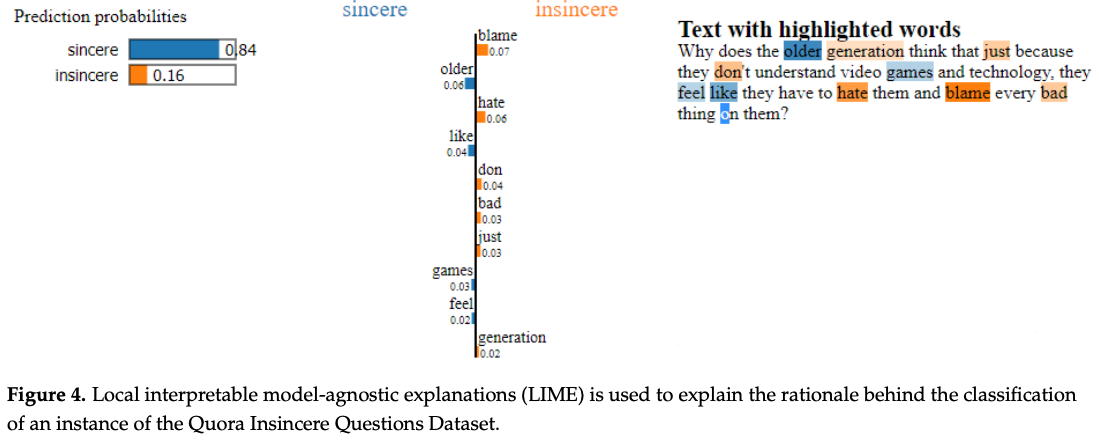
An example of feature attribution for text (from Explainable AI: A Review of Machine Learning Interpretability Methods):
An example of feature attribution for tabular data (from SHAP tutorial - official documentation):

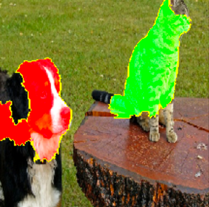
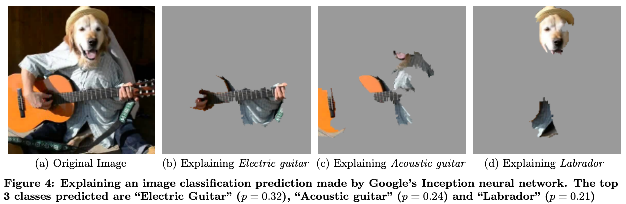
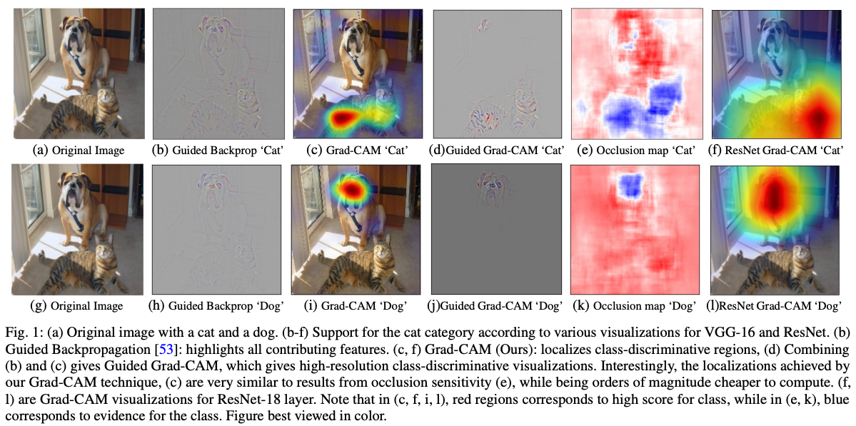
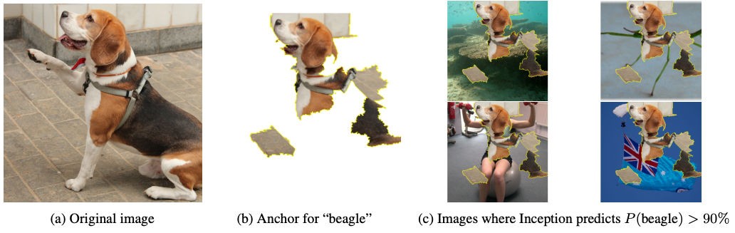
An example of feature attribution for a model that identifies a cat in a picture (from LIME’s GitHub):
What feature attributions are used for
The prominent use cases for feature attribution are:
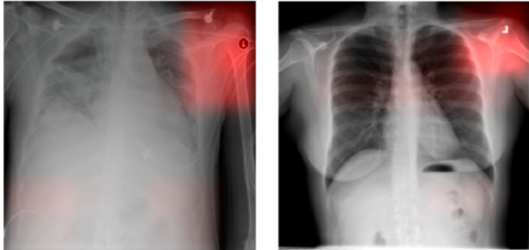
- Debug models: verify that models make predictions for the right reasons. For example, in the first picture below, a model predicts diseases in X-ray images based on the metal tags the X-ray technicians place on patients, not the actual disease marks (an example of spurious correlation).
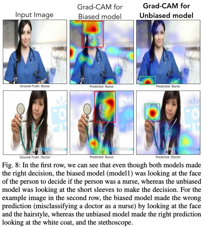
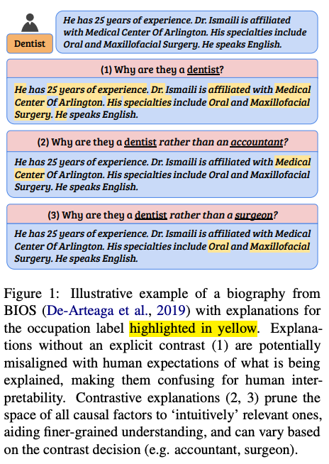
- Audit models: verify that models are not looking at attributes that encode bias (gender, race, among others) when making decisions. For example, in the second picture below, the middle column shows a gender-biased model that predicts professions by looking at the face in the image. The rightmost column shows where a debiased model looks to make predictions.
- Optimize models: simplify correlated features and remove features that do not contribute to predictions.
The figure below (source) is an example of feature attribution to debug a model (verify what the model uses to predict diseases). In this case, the model is looking at the wrong place to make predictions (using the X-ray markers instead of the pathology).
The figure below (source) is an example of feature attribution to audit a model. The middle column shows how the model predicts all women as “nurse”, never as “doctor” – an example of gender bias. The rightmost column shows a corrected model.
Where feature attribution is in relation to other interpretability methods
Explainability fact sheets defines the following explanation families (borrowed from Explanation facilities and interactive systems):
- Association between antecedent and consequent: “model internals such as its parameters, feature(s)-prediction relations such as explanations based on feature attribution or importance and item(s)-prediction relations, such as influential training instances”.
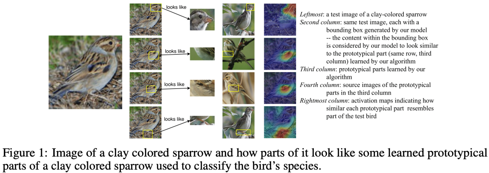
- Contrast and differences: “prototypes and criticisms (similarities and dissimilarities) and class-contrastive counterfactual statements”.
- Causal mechanism: “a full causal model”.
Feature attribution is part of the first family, the association between antecedent and consequent.
Using the framework in the taxonomy of interpretable models, we can further narrow down feature attribution methods as:
- Post-hoc: They are usually used after the model is trained and usually with black-box models. Therefore, we are interpreting the results of the model, not the model itself (c)reating interpretable models is yet another area of research). The typical application for feature attribution is to interpret the predictions of black-box models, such as deep neural networks (DNNs) and random forests. These models are too complex to be directly interpreted. Thus we are left with interpreting the model’s results, not the model itself.
- Result of the interpretation method: They result in feature summary statistics (and visualization - most summary statistics can be visualized in one way or another).
- Model-agnostic or model-specific: Shapley-value-based feature attribution methods can be used with different model architectures - they are model agnostic. Gradient-based feature attribution methods are based on gradients; therefore, they can be used only with models trained with gradient descent (neural networks, logistic regression, support vector machines, for example) - they are model specific.
- Local: They explain an individual prediction of the model, not the entire model (that would be “global” interpretability).
Putting it all together, feature attribution methods are post-hoc, local interpretation methods. They can be model-agnostic (e.g., SHAP) or model-specific (e.g., Grad-CAM).
Limitations and traps of feature attribution
Feature attributions are approximations
In their typical application, explanations have a fundamental limitation when applied to black-box models: they are approximations of how the model behaves.
“[Explanations] cannot have perfect fidelity with respect to the original model. If the explanation was completely faithful to what the original model computes, the explanation would equal the original model, and one would not need the original model in the first place, only the explanation.”
Cynthia Rudin — Stop Explaining Black Box Machine Learning Models for High Stakes Decisions and Use Interpretable Models Instead
More succinctly:
“Explanations must be wrong.”
Cynthia Rudin — Stop Explaining Black Box Machine Learning Models for High Stakes Decisions and Use Interpretable Models Instead
As we are going through the exploration of the feature attributions, we must keep in my mind that we are analyzing two items at the same time:
- What the model predicted.
- How feature attribution approximates what the model considers to make the prediction.
Therefore, never mistake the explanation for the actual behavior of the model. This is a critical conceptual limitation to keep in mind.
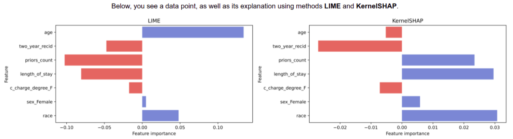
Because the explanations are approximations, they may disagree with each other. For example, in the figure below, LIME (left) and SHAP (right) disagree not only in the magnitude of features’ contributions but also in the direction (sign). This disagreement is more common than we may think. Refer to the excellent paper The Disagreement Problem in Explainable Machine Learning: A Practitioner’s Perspective for more details and how practitioners deal with this issue (the figure comes from the paper).
Feature attribution may not make sense
Feature attributions do not have any understanding of the model they are explaining. They simply explain what the model predicts, not caring if the prediction is right or wrong.
Therefore, never confuse “explaining” with “understanding”.
Feature attributions are sensitive to the baseline
Another conceptual limitation is the choice of a baseline. The attributions are not absolute values. They are the contributions compared to a baseline. To better understand why baselines are important, see how Shapley values are calculated in the Shapley values section, then the section on baselines right after it.
Feature attributions are slow to calculate
Moving on to practical limitations, an important one is performance. Calculating feature attributions for large images is time-consuming.
When used to help explain the predictions of a model to end-users, consider that it may make the user interface look unresponsive. You may have to compute the attributions offline or, at a minimum, indicate to the user that there is a task in progress and how long it will take.
User interactions are complex
The attributions we get from the feature attributions algorithms are just numbers. To make sense of them, we need to apply visualization techniques.
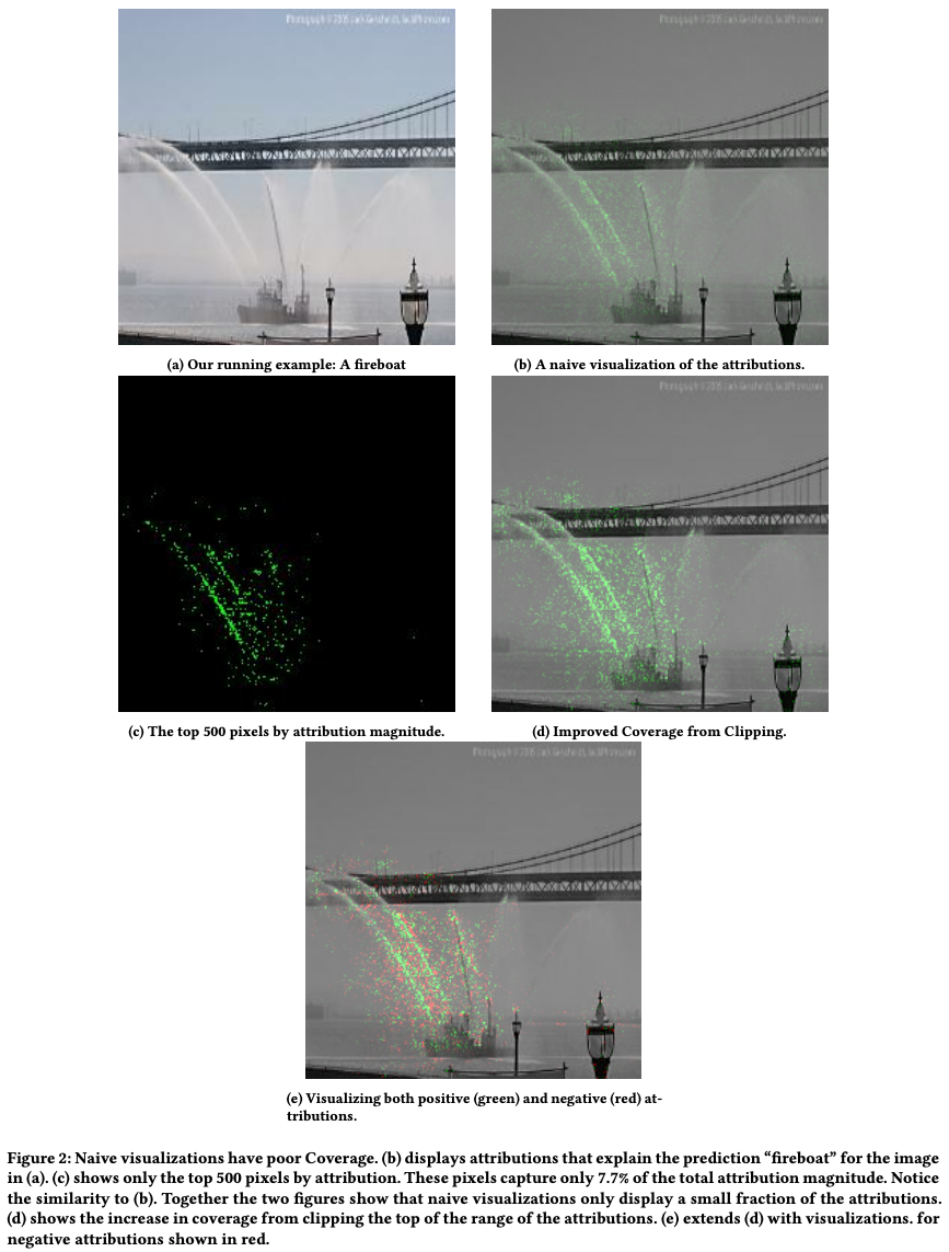
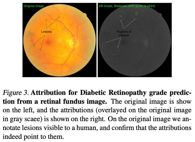
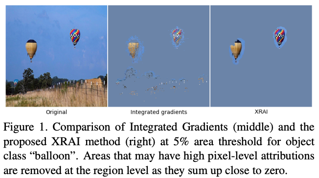
For example, simply overlaying the raw attribution values on an image may leave out important pixels that contributed to the prediction, as illustrated in figure 2 of this paper. Compare the number of pixels highlighted in the top-right picture with the one below it, adjusted to show more contributing pixels.
Showing all information at once to the users may also induce them to make more mistakes. For example, when showing the feature attributions overlaid to a medical image, this paper found out that it increased overdiagnosing of a medical condition. It points to the fact that just because we can explain something, we shouldn’t necessarily put that explanation in front of users without considering how it will change their behavior.
Well-known feature attribution methods
The following table was compiled with the article A Visual History of Interpretation for Image Recognition and the paper Explainable AI: A Review of Machine Learning Interpretability Methods.
Each row has an explanation method, when it was introduced, a link to the paper that introduced it, and an example of how the method attributes features. The entries are in chronological order.
A feature attribution example with SHAP
SHAP (SHapley Additive exPlanations) was introduced in the paper A Unified Approach to Interpreting Model Predictions. As the title indicates, SHAP unifies LIME, Shapley sampling values, DeepLIFT, QII, layer-wise relevance propagation, Shapley regression values, and tree interpreter.
Because of SHAP’s claim to unify several methods, in this section we review how it works. It starts with an example of SHAP for image classification, then explains the theory behind it. For a more detailed review of SHAP, including code, please see this article.
Example with MNIST
The code for the examples described in this section is available on this GitHub repository.
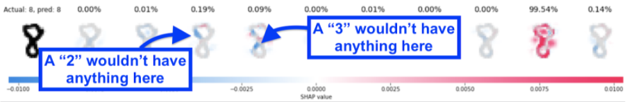
The following figure shows the SHAP feature attributions for a convolutional neural network that classifies digits from the MNIST dataset.
The leftmost digit is the sample from the MNIST dataset. The text at the top shows the actual label from the dataset (8) and the label the network predicted (also 8, thus a correct prediction). The next ten digits are the SHAP feature attributions for each class (the digits zero to nine, from left to right). At the top of each class we see the probability assigned by the network. In this case, the network gave the probability 99.54% to the digit 8, so it’s correct and very confident about the prediction.
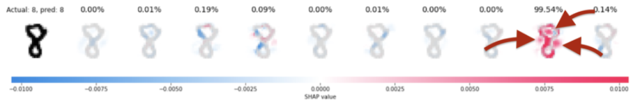
SHAP uses colors to explain attributions:
- Red pixels increases the probability of a class being predicted
- Blue pixels decrease the probability of a class being predicted
We can see that the contours of the digit 8 are assigned high probability. We can also see that the empty space inside the top loop is relevant to detecting a digit 8. The empty spaces to the left and right of the middle, where the bottom and top half of the digit meet are also important. In other words, it’s not only what is present that is important to decide what digit an image is, but also what is absent.
Looking at digits 2 and 3, we can see in blue the reasons why the network assigned lower probabilities to them.
Shapley values
SHAP uses an approximation of Shapley value for feature attribution. The Shapley value determines the contribution of individuals in interactions that involve multiple participants.
For example (based on this article), a company has three employees, Anne, Bob, and Charlie. The company has ended a month with a profit of 100 (the monetary unit is not essential). The company wants to distribute the profit to the employees according to their contribution.
We have so far two pieces of information, the profit when the company had no employee (zero) and the profit with all three employees on board.
| Employees | Profit |
|---|---|
| None | 0 |
| Anne, Bob, Charlie | 100 |
Going through historical records, the company determined the profit when different combinations of employees were working in the past months. They are added to the table below, between the two lines of the previous table.
| Employees | Profit | |
|---|---|---|
| 1 | None | 0 |
| 2 | Anne | 10 |
| 3 | Bob | 20 |
| 4 | Charlie | 30 |
| 5 | Anne, Bob | 60 |
| 6 | Bob, Charlie | 70 |
| 7 | Anne, Charlie | 90 |
| 8 | Anne, Bob, Charlie | 100 |
At first glance, it looks like Bob contributes 50 to the profit: in line 2 we see that Anne contributes 10 to the profit and in line 5 the profit of Anne and Bob together is 60. The conclusion would be that Bob contributed 50. However, when we look at line 4 (only Charlie) and line 6 (Bob and Charlie), we now conclude that Bob contributes 40 to the profit, contradicting the first conclusion.
Which one is correct? Both. We are interested in each employee’s contribution when they are working together. This is a collaborative game.
To understand the individual contributions, we start by analyzing all possible paths from “no employee” to “all three employees”.
| Path | Combination to get to all employees |
|---|---|
| 1 | Anne → Anne, Bob → Anne, Bob, Charlie |
| 2 | Anne → Anne, Charlie → Anne, Bob, Charlie |
| 3 | Bob → Anne, Bob → Anne, Bob, Charlie |
| 4 | Bob → Bob, Charlie → Anne, Bob, Charlie |
| 5 | Charlie → Anne, Charlie → Anne, Bob, Charlie |
| 6 | Charlie → Bob, Charlie → Anne, Bob, Charlie |
We then calculate each employee’s contribution in that path (this part is important). For example, in the first path, Anne contributes 10 (line 1 in the previous table), Bob contributes 50 (line 5, minus Anne’s contribution of 10), and Charlie contributes 40 (line 8 in the previous table, minus line 5). The total contribution must add to the total profit (this part is also important): Anne = 10 + Bob = 50 + Charlie = 40 → 100.
Repeating the process above, we calculate each employee’s contribution for each path. Finally, we average the contributions — this is the Shapley value for each employee (last line in the table).
| Path | Combination to get to all employees | Anne | Bob | Charlie |
|---|---|---|---|---|
| 1 | Anne → Anne, Bob → Anne, Bob, Charlie | 10 | 50 | 40 |
| 2 | Anne → Anne, Charlie → Anne, Bob, Charlie | 10 | 10 | 80 |
| 3 | Bob → Anne, Bob → Anne, Bob, Charlie | 40 | 20 | 40 |
| 4 | Bob → Bob, Charlie → Anne, Bob, Charlie | 30 | 20 | 50 |
| 5 | Charlie → Anne, Charlie → Anne, Bob, Charlie | 30 | 40 | 30 |
| 6 | Charlie → Bob, Charlie → Anne, Bob, Charlie | 60 | 10 | 30 |
| Average (Shapley value) | 30 | 25 | 45 |
In this example we managed to calculate each individual’s contribution for all possible paths in a reasonable time. In machine learning, the “individuals” are the features in the dataset. There may be thousands or even millions of features in a dataset. For example, in image classification, each pixel in the image is a feature.
SHAP uses a similar method to explain the contribution of features to a model’s prediction. However, calculating the contribution of each feature is not feasible in some cases (e.g. images and their millions of pixels). The combination of paths to try is exponential (factorial, to be precise). SHAP makes simplifications to calculate the features’ contributions. It is crucial to remember that SHAP is an approximation, not the actual contribution value.
The importance of the baseline
In the example above, we asked “what is each employee’s contribution to the profit?”. Our baseline was the company with zero employees and no profit.
We could have asked a different question: “what is the contribution of Bob and Charlie, given that Anne is already an employee?”. In this case, our baseline is 10, the profit that Anne adds to the company by herself. Only paths 1 and 2 would apply, with the corresponding changes to the average contribution.
SHAP (and other feature attribution methods) calculate the feature contribution compared to a baseline. For example, in feature attribution for image classification, the baseline is an image or a set of images.
The choice of the baseline affects the calculations. Visualizing the Impact of Feature Attribution Baselines discussed the problem and its effect on feature attribution.
Appendix - interpretability vs. explainability
Ajay Thampi’s Interpretable AI book distinguishes between interpretability and explainability this way:
- Interpretability: “It is the degree to which we can consistently estimate what a model will predict given an input, understand how the model came up with the prediction, understand how the prediction changes with changes in the input or algorithmic parameters and finally understand when the model has made a mistake. Interpretability is mostly discernible by experts who are either building, deploying or using the AI system and these techniques are building blocks that will help you get to explainability.”
- Explainability: “[G]oes beyond interpretability in that it helps us understand in a human-readable form how and why a model came up with a prediction. It explains the internal mechanics of the system in human terms with the intent to reach a much wider audience. Explainability requires interpretability as building blocks and also looks to other fields and areas such as Human-Computer Interaction (HCI), law and ethics.”
Other sources treat interpretability and explainability as equivalent terms (for example, Miller’s work and Molan’s online book on the topic).
This article uses “interpretability” as defined in Ajay Thampi’s book. We distinguish between interpretability and explainability to not involve aspects of displaying the interpretation of a model’s prediction to end-users. This would add to the discussion other topics such as user interface and user interaction. While important for the overall discussion of ML interpretability and explainability, these topics are not relevant to the scope of this work. However, we preserve the original term when quoting a source. If the source chose “explainability”, we quote it so.
Therefore, when we discuss “interpretability” here, we mean the interpretation that is shown to a machine learning practitioner, someone familiar with model training and evaluation. We discuss interpretability in a more technical format with this definition in place, assuming that the consumer of the interpretability results has enough technical background to understand it.